LATEST RELEASE: BetaMatch version 3.4.0 - Get it here!

A quick optimization example

This is a brief step by step introduction to the optimization feature of BetaMatch.

1. Start BetaMatch. We will use the example file called ‘DualBand’ for this example. If the title says ‘DualBand (Demodata)’ the correct curve is loaded. If not go to “Help –>Load demo data... ” in the help menu and select ‘DualBand’ from the list of example files. Your window should look like this:

2. The electrical delay must be entered if it is not equal to 0 pS. It is very important to compensate for any electrical delay that is not present in the Touchstone data. If the reference plane is not correct all calculated networks will be wrong. For this example move the cursor to highlight (blue circle) El Delay in the window that shows the network. Left-click and enter 50.0ps in the pop-up window:

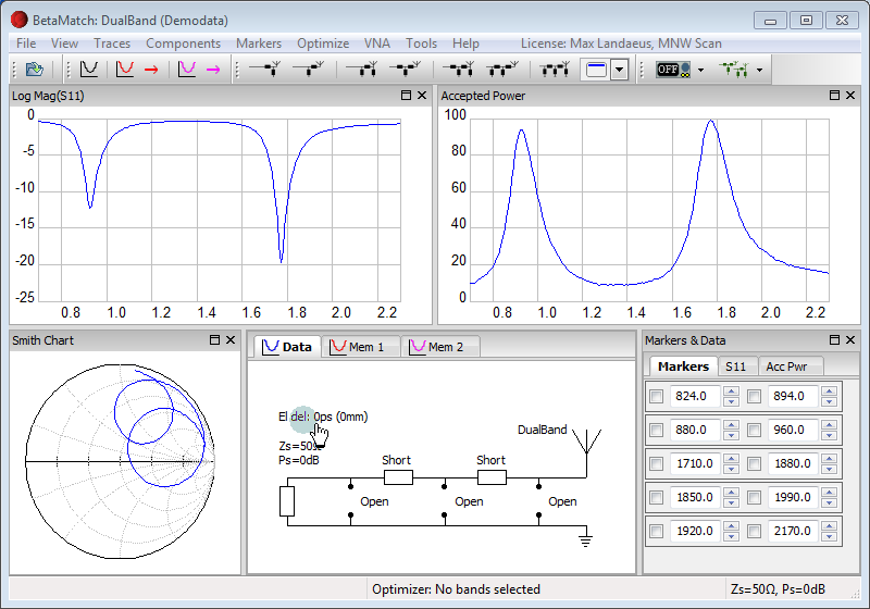
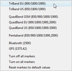
3. The optimizer needs to be told which frequencies to optimize for. This is done by selecting bands from the Markers menu or by setting pairs of markers in the Marker & Data window.

   For this example select “Markers –> Triband EU ” from the menu. This will set the 900, 1800 and 1900MHz bands as frequency bands for our optimization.

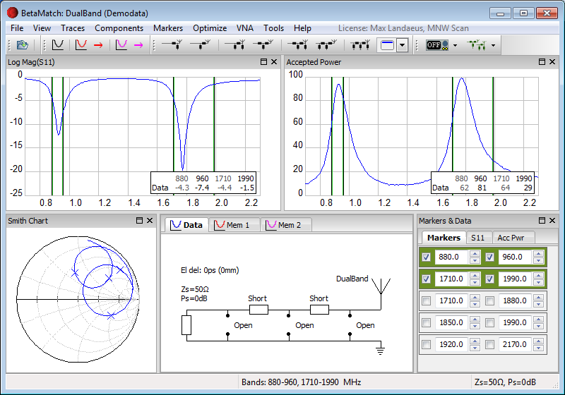
Markers will now be shown as crosses (‘x’) in the Smith Chart and as vertical lines in the other plots. In Markers & Data window the new markers will be ticked to indicate that they are active.

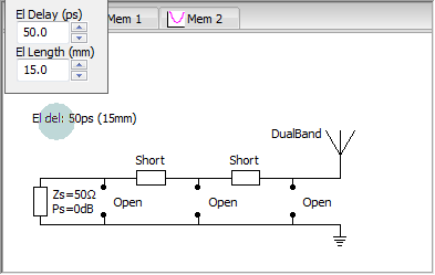
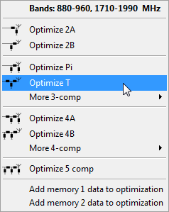
The frequency ranges for optimization will be 880 - 960 MHz and 1710 - 1990 MHz. There are only two bands because of the overlap between the 1800MHz and 1900MHz bands. The frequencies that will be used for optimization are shown in the right hand side of the status bar and also at the top of the “Optimize” menu.

4. Now everything is ready to start the optimization. The optimizer can be started either from the Optimize menu or the Optimizer Tool-bar. Open the ‘Optimize’ menu. Notice that the frequency bands for optimization are displayed on the top row.

The optimization is started by selecting the desired network from the menu. Select Optimize T (“Optimize –> Optimize T”).

After a moment the best matching T-net is shown in the network plot and the data is shown in the plotted curves.

The results at marker frequencies for |S₁₁| and Accepted Power is displayed under respective tab in the Markers & Data window.

In order to compare the optimized results with the original select ‘Show original’ from the Memory menu. The original results are displayed in the plots in black colour and the optimized results in blue. The screen should now look something like this:

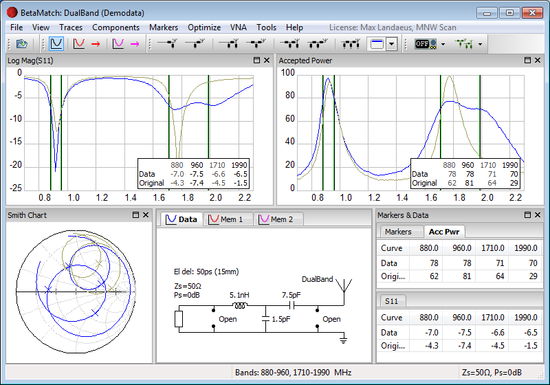
The data in the Accepted power tab shows that the without matching network this antenna has the worst performance at 1990MHz where the accepted power (the power into the antenna) is 29%. After the optimization the T-net will improve the accepted power to 70% at this frequency.