LATEST RELEASE: BetaMatch version 3.4.0 - Get it here!

Tolerance Analysis

With the Tolerance Analyzer it is easy to estimate the sensitivity and accuracy of the current matching network with respect to component tolerances.

To start the Tolerance Analyzer either select Tools Menu –> Show Tolerances or press <CTRL-D>.

The Tolerance Analysis will take the current matching network and run a Monte Carlo simulation using the actual component tolerances as given by the manufacturers. For ideal components the tolerances can be set in the Tolerance Settings (see below on how to set the various simulation parameters).

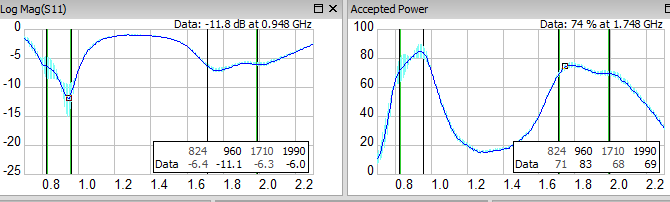
When the simulation is finished the data traces in the log |S₁₁| and the Accepted Power plots will be shadowed with vertical bars showing the range (this range can be set in Tolerance Settings. The default value is 99.73% (which corresponds to ±3σ for a normal distribution):

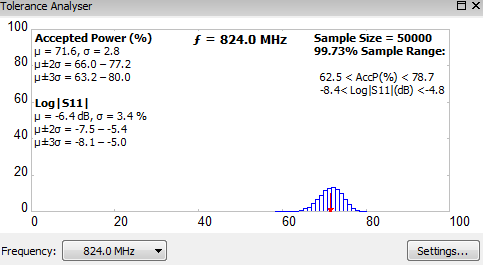
More accurate data for each frequency point can be read from the Tolerance Plot which looks like this:

This plot shows a histogram of the distribution of the Accepted Power at a given frequency.

The frequency for the Tolerance Plot can be set to Follow Cursor (which means that the frequency will be the same as the linked cursor data in the other plots) or to any of the currently active marker frequencies (the marker has to be turned on).

On the left side of the plot mean value(μ), standard deviation (σ) and interval for the ±2σ and ±3σ-ranges are displayed for Accepted Power and Log|S₁₁|. All these values are based on the calculated mean and standard deviation and may not always be accurate. This can happen if, for instance, the final distribution is not close to a normal distribution, component tolerances are very wide or the population is too small.

Note that ±2σ and ±3σ-ranges are truncated to stay within 0 - 100% for the accepted power and to be below 0 for Log|S₁₁|.

On the right side of the tolerance plot Sample Size together with the upper and lower Accepted power and log|S₁₁| values for the user defined range (see Tolerance Settings on how to adjust the user interval) are displayed on the right side. These values are based on the actual sample population and not on calculated entities such as mean value and standard deviation.

Note that if the Accepted Power plot is changed to use Log-scale the units in the Tolerance plot will also change accordingly.

The settings button brings up the Tolerance Settings window from BetaMatch options:

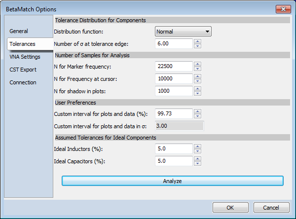
There are a number of options that can be set that controls the Tolerance Analysis:

• The component distribution function can be set to one of: uniform, normal, truncated normal or triangular.

• If one of the normal or truncated normal distribution functions is selected the width of the function is controlled by the parameter “Number of σ at tolerance edge”. For instance, setting this parameter to 3 means that the outer tolerance range will coincide with the 3σ-range (99.7% of the components).

• There are three different population sizes that are used for different Monte Carlo simulations. They can be individually be set under “Number of samples for analysis”. The reason to use three different populations is to find a reasonable compromise between accuracy and speed for various situations:

  • N for Marker frequency: This is the population size used when a marker frequency is selected in the frequency selection box. Since this simulation only is run at one single frequency the population can be set rather high.
  • N for Frequency at cursor: This is the population size used when the frequency is set to follow the linked cursor data. Since this simulation will be repeated as soon as the cursor moves to a new frequency the population size is set a bit lower in order to keep the plots responsive.
  • N for shadow in plots: This simulation is run for all frequencies when the tolerance analysis is started or updated (i.e. by a component change). The population for this case is set rather low in order to not delay the update. Since the results only are used to plot the vertical bars that indicates the tolerance intervals the need for accuracy is less than for the other cases.
  
  

• The Custom interval for plots and data parameter is used to set the range for Accepted Power and Log |S₁₁| values that are displayed on the right side of the Tolerance Window. This value is also used to display the range in the plots (the shaded portion).

  The value is always entered as a percentage of the total range and for convenience the same value as number of σ:s is shown in the field below.

• Under Assumed Tolerances for Ideal Components the tolerances for ideal inductors and capacitors can be set.

  For other components the actual tolerance given by the manufacturer will always be used. Note that some component series are divided into sub-series with different tolerance level. In order to see differences change the component series to a series with tighter/looser tolerances.

• The Analyze button can be used to force a new tolerance simulation when the settings have been changed.