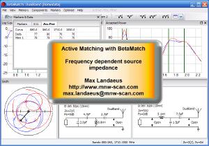
LATEST RELEASE: BetaMatch version 3.4.0 - Get it here!

Traces

Operations that applies to the active data trace and the Memory traces can be found in the Traces Menu:

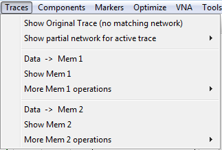
Traces Menu and the Show Memory Toolbar

Active Data Trace

The Show original and Partial Network options operates on the active data trace.

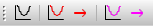
Show Original Trace... displays the current active (data) trace as it is before any matching network has been applied (but with any electrical delay). This trace can also be shown and hidden from the leftmost button in the ‘Show Memory Toolbar’ (see above).

Show partial network for active trace: Shows data data traces from “inside” the matching network. This can be used to spot differences between a calculated network and an actual physical network. For a detailed description see Partial Network Plots below.

Memory Curves

There is often a need to compare different results. The most common are the following:

1. Data with and without a matching network (how much does the matching improve?).
2. Same data with different matching networks (finding the best matching topology).
3. Different data with same matching network (e.g. flip phone in opened and closed positions).
4. Data with calculated matching network and data with implemented matching network (correction for deviations - e.g. electrical delay).
5. Different data with different matching networks (e.g. different antenna structures with optimized matching).

For this purpose there are two memory curves available. The functions for both these curves are:

• Data –> Memory: This stores the current data (including current electrical delay and matching components).

• Show Memory: Toggles whether this memory should be shown in the plots or not.

  Note: It is possible to turn off the display for all curves except for current data curve in the Smith Chart (from Smith Chart’s context menu). This is often convenient since the Smith Chart often becomes to cluttered when to many curves are displayed.

• Add electrical delay to memory: This adds the current electrical delay to the memory curve and (temporarily) overrides any electrical delay that was originally stored. When toggled to off the electrical delay will be restored to the original value.

• Add matching to memory: When on the current matching network to the memory curve, and (temporarily) override any originally matching that was stored. When this option is turned off the matching that was stored originally will be restored.

• Memory to Data: Overwrites the current data with the data from memory. Note that this will change the data and the network. The component series may also change if the memory was using a different component series.

• Swap Memory and Data: Exchanges the data and memory curves. Network and components series are also interchanged.

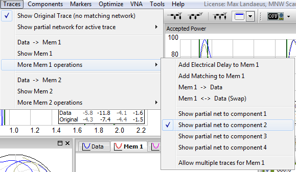
Data –> Memory and Show Memory are available directly from the Trace Menu and also from the Memory Toolbar. The other options can be found the submenu Trace Menu –> More Mem 1 (Mem 2) operations:

More Memory operations for Memory 1

Information about the matching, electrical delay, loaded data etc can be viewed by clicking the Mem1 and Mem2 in the graphic network. Note that it is only possible to change the component values in the ‘Data’ window. The ‘Memory’ windows are not editable and it is not possible to change the network. It is, however, possible to copy, save and print the ‘Memory’ networks the usual way (see Context Menu for Plots ).

The network window is highly reconfigurable. It is possible to relocate any of the tabs by dragging and dropping it. An example of what is possible:

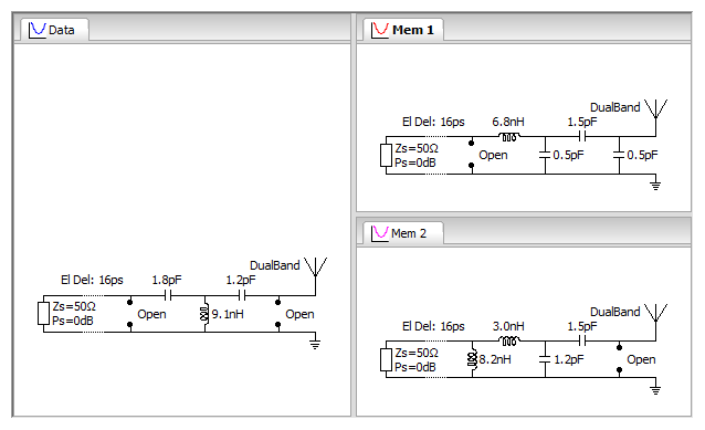
The tabs for data and memory networks can be dragged and rearranged.

Partial Network Plot: View data inside the network

Sometimes it is useful to be able to see the results “inside the matching network”, that is, before all components have been added. This can be a great help when moving from the calculated results to actually soldering the components onto the prototype.

These results can also be viewed by only entering part of the network into BetaMatch. However, it is much more convenient to use the built in “Partial Network Plot” functionality described here.

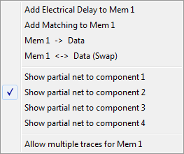
These plots are available both for the Active Data Trace as well as for the memory traces. The plots are activated from the Memory Menu –> Show Partial Network for Active Trace and from Memory Menu -> More Mem1/Mem2 operations.

To view a trace from within the network select Traces –> Show partial network for active trace. The sub-menu looks like this:

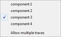
Select after which component you would like to see the data trace. A triangular marker shows where the data is plotted from.

The data will be the same as if the remaining components between the selected and the source is set as “short” and “open”.

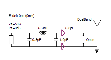
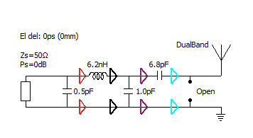
Network with ‘Component 2’ selected.

The data plotted for the network above will be the same as for the network below where components 3, 4 and 5 have been removed:

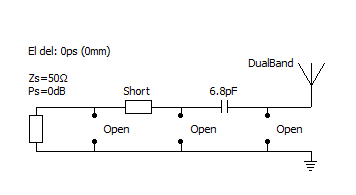
The network that corresponds to above where ‘Component 2 was selected.

The data traces will have the same colour as the triangular marker in the network:

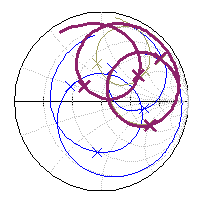
All plots that can show the data trace can also display partial net plots: LogMag, Accepted Power, Smith, VSWR, Phase, Real(Z), Im(z) and Q-Factor.

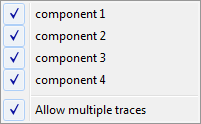
Normally only one partial trace can be displayed and when the user selects another component the first trace will automatically unselected. If there is a need to display more than one trace at the same time select Allow Multiple Traces from the menu. Then any combination of traces can be selected (and the user must manually de-select any traces that he don’t want to display).

For Memory 1 and Memory 2 this functionality is available from Traces –> More Mem 1 (Mem 2) Operations. The same options as for the active trace is available here: