LATEST RELEASE: BetaMatch version 3.4.0 - Get it here!

Screen Graphics and User Interface

This section will describe the available plots, windows and some general information on how the user interface works.

Available Plots

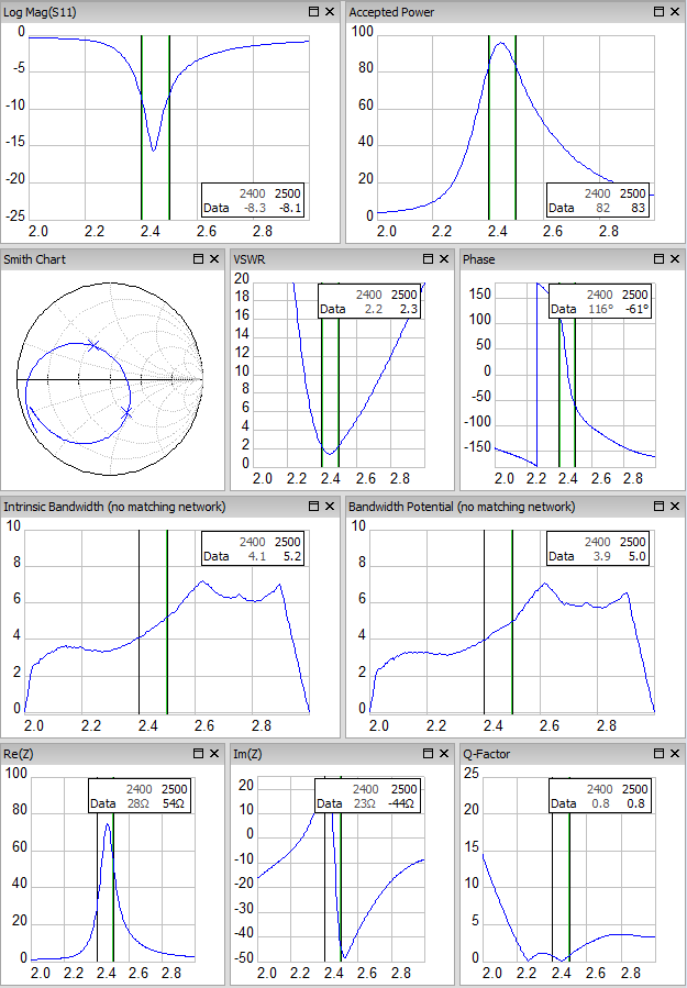
The following plots are currently available:

• Return Loss: Shows |S₁₁| in dB
• Smith Chart
• Accepted Power: Shows the power accepted by Z _Load (the Antenna). Linear or logarithmic scale can be selected from the context menu.
• VSWR
• Intrinsic Bandwidth (see here).
• Bandwidth Potential (see here).
• Phase (of S11)
• Re(Z)
• Im(Z)
• Q-Factor (|Im(Z)/Re(Z)|)

The general options and settings described in this section also apply to the plots that are available from the Tools menu: Conversion Plot, Channel Plot and Skin Effect Plot.

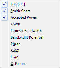
All trace plots can be hidden and shown from the View menu. They can also be maximized, restored and closed from the icons on the caption bar:

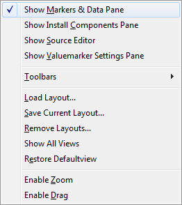
Other windows can be accessed via the View Menu. The toolbars can also be shown and hidden from this menu. Layouts can be loaded and saved as well:

Cursor Data

When the cursor is moved over any of the plot window a square marker is showing the nearest point on the nearest curve. Data for this point is displayed at the top right corner of each plot.

If possible the corresponding data point is shown in the other plots as well.

This linking of cursor data can be turned on and off in the context menu in any of the plots.

Zoom & Drag

All plots can be zoomed and dragged. When zoom-mode is ON the cursor is changed from a cross to a magnifier glass. When drag is enabled the cursor is changed to a hand-cursor.

The plots can be zoomed in two ways:

• Move the cursor to the plot, hold down the Ctrl-key and use the mouse to make a window while holding down the left mouse-button.
• Select View –> Enable Zoom from the menu. Zoom is now on by default and the plots can be zoomed by just holding down the left mouse-button and making a window.

Dragging can be done by:

• While holding down the Shift-key press the left mouse-button and move the mouse to drag.
• Select View –> Enable Drag from the menu. Drag is now on by default and the plots can be dragged by just holding down the left mouse-button and making a window.

Zoom and Drag are intended to be used to read values with enhanced accuracy therefore they are non-persistent. This means that the original plot settings will be restored when the plots are redrawn (e.g. by double-clicking or by changing the matching network).

Context Menu for Plots

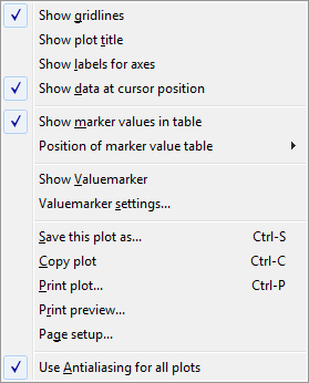
Right-click on any of the plots to show the context menu. The context menu consists of some items that are common to all the plots and some items that are unique to each plot. The common options are:

Most of these are quite obvious. Show grid-lines, Show plot title and Show labels for axes are available in all plots except for Smith Chart. These settings are global and will immediately change all trace (data) plots except for the Smith Chart. They are also persistent and the current settings will be restored next time BetaMatch is started.

The Show data at cursor position toggles the linked cursor data on and off.

Show values in table shows/hides the table that shows data values at marker frequencies in each plot.

Position of valuetable gives the choice to set the position of the table. Choices are: Upper left, upper right, lower left and lower right.

The options Show Valuemarker toggles the valuemarker on or off and the Valuemarker settings... opens a window where the value of this marker can be set. See Valuemarker for more information.

Save this plot as... gives the option to save the current plot in JPEG, PNG, bitmap and some other formats. This command is also accessible via shortcut Ctrl-S.

Copy plot copies the current plot into the clipboard. The plot can then be pasted into other documents. Shortcut: Ctrl-C

There are also options to print, preview and also to setup options for the printout (‘Page setup...’). Note that ‘Page setup...’ only sets the value for the current plot (e.g. changing the settings for VSWR plot will not change the settings for the Return Loss or any other plots).

The last option, Use anti-aliasing for all plots will increase the quality of all plots when turned on. Note however, that this functionality also uses more computational power and that updates of the plots may be slower. Normally this is not noticeable, but may be so on a slower computer and if many plots are displayed simultaneously. When BetaMatch is connected to VNA is another occasion when the difference in plotting speed may be noticed. This option is persistent and the last used value will be restored whenever BetaMatch is started.

Accepted Power Plots

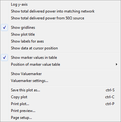
The Accepted Power Plot has a few more options in the context menu:

• Log y-axis: Shows the accepted power in dB instead of %.
• Show total delivered power into matching network: Shows the amount of power delivered from the source that is accepted by the antenna + matching network. This will show the correct amount even if the source impedance in not 50Ω or not constant. The curve will be shown as a dashed line.
• Show total delivered power from 50Ω source: Same as above but assuming that the source impedance is constant 50Ω regardless of setting.

All the options above are persistent and will be remembered between runs.

Smith Chart Plot

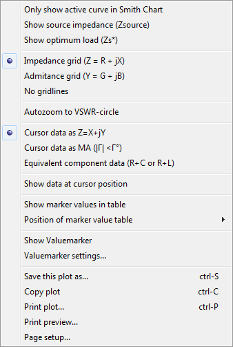
The Smith Chart has a few additional options in the context menu (items marked “persistent” will retain the setting between BetaMatch startups):

• The first group sets what data to show:

  Only show active curve in Smith Chart (persistent): This option hides all memory curves in this plot even when they are enabled.

  Show source impedance (Zsource) (persistent): Plots the current impedance of the source. Useful when the impedance is not 50Ω.

  Show optimum load (persistent): This will show the best load for the current source impedance (i.e. the conjugate of the source impedance).

• Impdance grid (Z=R+jX), Admitance grid (Y = G + jB) and No gridlines (persistent):switches between impedance, admittance grid or to turn the grid off.

• Autozoom to VSWR-circle: When set to on the Smith Chart will automatically zoom and only show the area inside the circle defined by the current VSWR value (set by the Value marker). This option will only have effect when the Show Valuemarker is turned on (see Valuemarker).

• Cursor Data (persistent): This sets the output format of the Cursor Data. There are three different format to choose from: Rectangular (real and imaginary), Polar (magnitude and angle) or as Equivalent Component Data (R+C or R+L).

See Context Menu for Plots for a description of the other options in this menu.

The following of the options above are persistent and the last setting will be restored when BetaMatch is started:

Intrinsic Bandwidth and Bandwidth Potential Plots

Intrinsic Bandwidth is the 6dB-bandwidth obtained when the trace is matched to 50Ω for each frequency point. The match is achieved by setting the load impedance, Z_load(ƒ), to Z^*_trace(ƒ) for each frequency point (ƒ).

Bandwith Potential is similar to the Intrinsic Bandwidth above, but an ideal 2-component network is used to achieve an exact match to 50Ω match instead of a fixed impedance.

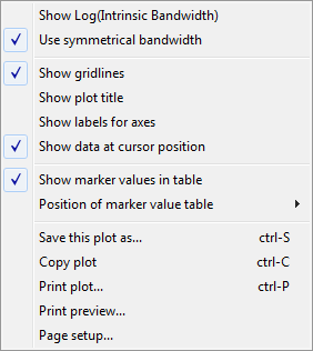
Intrinsic Bandwidth and Bandwidth Potential plots have two extra options in the right-click menu:

• The first option is to show the values in dB (Show Log(...)) instead of in % (linear). Persistent, the last setting will be restored when BetaMatch is started.

• The other option is to Use symmetrical bandwidth, which may need some clarification: By symmetrical bandwidth at frequency ƒ I mean the bandwith obtained when ƒ is forced to be the center frequency in the band. That is:

  BW_symmetrical = 2dƒ / ƒ_c, where dƒ = min(ƒ_c - ƒ_lower, ƒ_upper - ƒ_c).

  Use symmetrical bandwidth is persistent and the last value will be restored when BetaMatch is started.

User Interface

The user interface is very flexible and you can move, dock/undock, resize and open/close most of the panels.

It is possible to save the current view and load it later or have it automatically loaded when BetaMatch is started. This is done from the View Menu.

These options are in the third section of this menu:

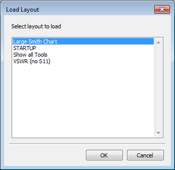
• Load Layout: Use this option to select and load a previously saved layout. In the list below there are 4 saved images: One with a large Smith Chart, another where VSWR is shown instead of |S₁₁| and a third where all the conversion plots from the Tools menu are shown. The layout called ‘STARTUP’ will be automatically loaded whenever BetaMatch is started (in this case it is the same as the view called ‘VSWR’).

  
  
  

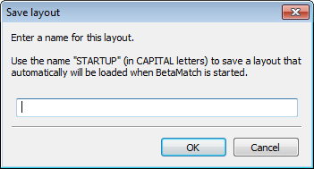
• Save Current Layout: This option lets you save the current layout. Enter a descriptive name in the text box and press OK to save the layout. If you want BetaMatch to automatically load the current layout when it is started save it under the name ‘STARTUP’ (must be capital letters).

  
  
  

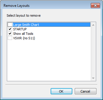
• Remove Layouts: Layouts can be deleted by ticking the appropriate boxes and pressing OK. Press Cancel to close the window without removing any layouts. If you remove the ‘STARTUP’ layout BetaMatch will use the factory default layout when it is started.

  
  
  

• Show All Views: All available windows will be displayed. This will be rather messy, but can be useful when designing a new layout: First display all windows and then close the ones that are not needed.

• Restore Defaultview: A shortcut that will load the ‘STARTUP’ view if it exists otherwise the factory default layout will be shown.

Note

It is currently not possible to guarantee compatibility of the saved layouts between different versions of BetaMatch. That means that it may not be possible to correctly load old layouts after BetaMatch has been updated to a later version.

If this happens it is recommended to delete the old layouts via the View ‣ Remove Layouts in the menu and then create and save the layouts again in the new version of BetaMatch.