LATEST RELEASE: BetaMatch version 3.4.0 - Get it here!

Various useful utilities are collected under the Tools Menu.
There are some graphical tools intended to make it easy to interactively look up and convert between different entities. There are, to mention a few, conversion charts between “|S11| and VSWR”, between “dBm and mW” and of “Skin depth vs frequency for various materials”.
In addition there is also a tool that extracts and creates text-files with tabular data from a directory with Touchstone files see Batch Export Data.
The plots in this section has the same functionality as the other plots:
See Description of the Plots for more details regarding the global plot options and settings.
There are three entries Tools Menu :
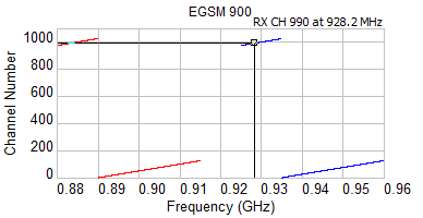
Use these plots to translate between channel numbers and frequency for GSM and WCDMA bands. TX and RX channels are plotted in red and blue colour respective. Channel number and frequency will be printed to the upper right of the graph for the point closest to the cursor (e.g. RX channel 990 at 928.2MHz in the figure below).
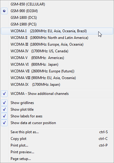
The plotted band is changed from the context menu (right click on the graph) and there is a choice between the most common GSM and WCDMA bands.
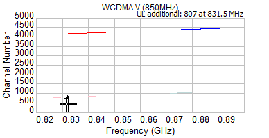
Some WCDMA bands have additional channels that are outside the normal channel numbering. The option Show extra WCMDA channels in the context menu switches the display of these channels ON or OFF. When shown the additional channels are displayed in light red (TX channels) and light blue (RX channels) as shown in the plot of WCDMA band III below:
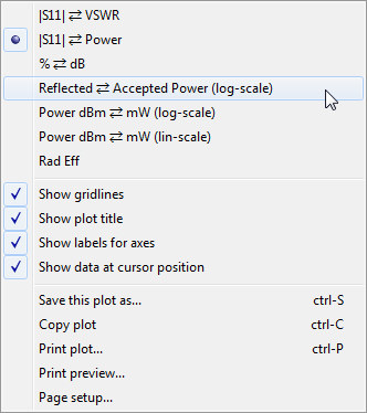
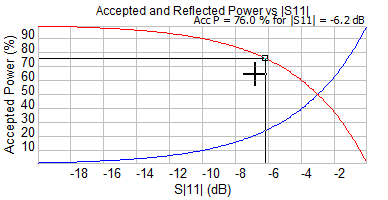
This collection of graphs makes it easy to convert between various entities such as |S11|, VSWR, reflected and accepted power etc. Select conversion graph from the context menu (see figure below) and move the marker to the data point of interest. The result can be read to the right above the plot area.
The two first graphs (“|S11| vs VSWR” and “|S11| vs reflected and accepted power”) shows the relation between matching and power into the antenna. For example, in the figure below you can see that with an return loss of -6.2dB there will be 62% accepted power going into the antenna and the remaining 38% will be reflected.
Note
Conversions
It is also possible to use the Valuemarker to convert between |S11| (dB), VSWR, Reflected Power, Accepted Power and Reflection Coefficient. For more details see the Valuemarker section.
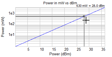
The next four plots are basically various conversion between logarithmic and linear power values that can be handy. As an example, the reading in the plot below shows that 28dBm corresponds to 630mW.
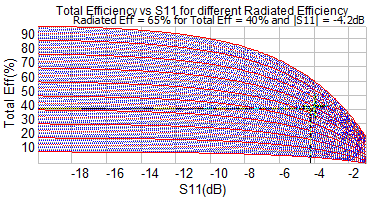
Rad Efficiency (Total efficiency vs |S11| for different Radiated Efficiency**): This plot is intended to be used as a quick way to estimate the radiated efficiency when both |S11| and total efficiency are available. In the figure below, for example, the return loss is -4.2dB and the measured efficiency (from your 3D-chamber) is 40% then the radiated efficiency is 65%. That means that the there is 100-65=35% ohmic losses caused by antenna and platform and that efficiency can never be higher than 60% regardless of how well matched the antenna is. If a higher efficiency is a requirement it can only be achieved after some of the losses have been identified and eliminated.
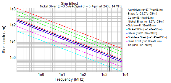
This plot shows how the skin depth varies with frequency for various materials. The legends at the right side shows the different materials and the conductivity used to calculate the skin depth. To get more area for the plot it is possible to hide the legends by unticking the Show Legends option in the context menu.
In the figure below the reading shows that the skin depth for Nickel Silver at about 2450MHz is 5.4 micrometer.